 The Academy

INSTRUCTOR: WILLIAM PALM
The students used Matlab for computational assistance and to run a simulation of the system using the linearized model. They then used Working Model to simulate the performance of their controller using the more realistic nonlinear dynamics model. The project was very successful. If their design did not satisfy the performance specifications, they could see the system behaving badly in an unstable manner. It is possible to test the design using traditional methods based on solving the nonlinear equations and plotting the system's position as a function of time, but using Working Model was far more easy, more interesting, and more motivating.
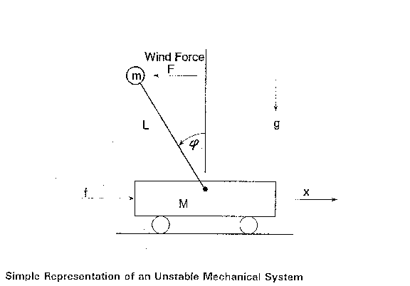
Assumptions. We will assume that system consists of two masses: M, the base mass, and m, the mass of the rotating component. The center of mass of m is a distance L from its pivot point. We will assume also that the time constant of the base thruster (which supplies the force f) is small compared to the other time constants. This means that the thruster acts almost "instantaneously" to produce the force f. We also assume that a random wind force F acts on the mass m.
Linearization. The model derived in class is nonlinear, but can be linearized if we assume that phi and its time derivatives are small. The linearized model is

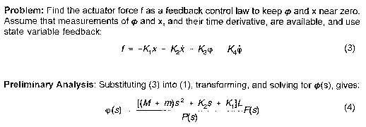
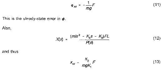
which is a steady-state error in x.
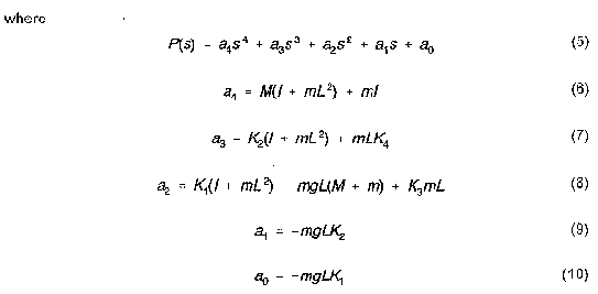
Numerical values: The given system values are: m=2.268 kg, M=0.008 kg, L=0.394 meter, |=0.102 kg-m2, and g=9.81 m/s2. With these values, the coefficients of the characteristic equation, given by (6) - (10) become
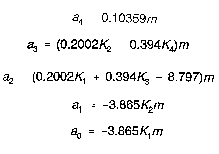
These equations can be used to find the feedback gains, given the desired roots.
Example and Test Case: Suppose we want the dominant time constant to be 1 second, with no oscillations. Thus the dominant root must be s = -1. Suppose we want the secondary roots to be separated from the dominant root by a factor of 10; that is, at s = -10. Then P(s) must be
Comparing this with (5), we can solve for the required gain values: K1 = -26.8, K2 = -34.84, K3 = 122.7, and K4 = 25.84. Thus (phi)ss = -0.045F, and xss = -0.206F.
Assignment (Part 1): Find the gain values and (phi)ss and xss for the roots assigned to you in the assignment sheet. Then use Matlab to obtain a plot of the step response of (phi) and x for F = 1.
Assignment (Part 2): We want to see how well the controller performs when the mass m is 10% of its nominal value (for example due to fuel consumption). Assume that the fuel tank is symmetric about the center of mass, so that the cg location does not change. Then L is constant, and I = 0.102m/2.268 = 0.04497m. Defining (delta) = 2.268 - m and rearranging the characteristic equation into the standard root locus form, we obtain
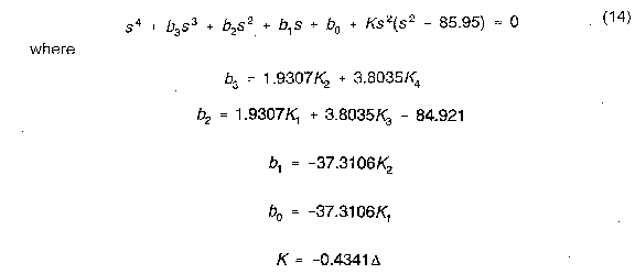
If we let m vary from 2.268 to 0.1(2.268), then (delta) varies from 0 to 0.9(2.268), and K varies from 0 to -0.4341(0.9)(2.268) = -0.886. Thus we are interested in the root locus for -0.886 <= K <= 0.
Use your values of the gains computed in part 1 to obtain the root locus plot with Matlab, for two cases:
Case 2: -0.886 <= K <= 0
For case 2, what is the percent change in t (the dominant closed-loop time constant) from its design value of t = 1? What is the maximum oscillation frequency?
Assignment (Part 3): a) Use your gain values and the Working Model file BALNCBAT.WM to simulate your controller design in Working Model. You must change the gain values used in BALNCBAT.WM from their default values to the values you computed. You must also change mass values and dimensions, and the random wind force to a constant force equal to 1. Save the meter values in Working Model, and use Excel to plot phi(t) and x(t) vs. t. Compare these plots with those you generated in Part 1 (which are based on the linearized model).
b) Reset the wind force to its original random function, and run the simulation of your controller. How well does it perform? Give a reason for your answer.