![]()
![]()
The objectives of this module are to:
The four-bar linkage is the simplest possible closed-loop mechanism, and has numerous uses in industry and for simple devices found in automobiles, toys, etc. The device gets its name from its four distinct links (or bars), as shown in Figure 1. Link 1 is the ground link (sometimes called the frame or fixed link), and is assumed to be motionless. Links 2 and 4 each rotate relative to the ground link about fixed pivots (A0 and B0). Link 3 is called the coupler link, and is the only link that can trace paths of arbitrary shape (because it is not rotating about a fixed pivot). Usually one of the "grounded links" (link 2 or 4) serves as the input link, which is the link which may either be turned by hand, or perhaps driven by an electric motor or a hydraulic or pneumatic cylinder. If link 2 is the input link, then link 4 is called the follower link, because its rotation merely follows the motion as determined by the input and coupler link motion. If link 2 is the input link and its possible range of motion is unlimited, it is called a crank, and the linkage is called a crank-rocker. Crank-rockers are very useful because the input link can be rotated continuously while a point on its coupler traces a closed complex curve.
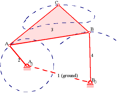
Figure 1: Four-bar linkage showing paths traced by moving pivots A and B, and coupler point C.
A fundamental concept in modeling a linkage is the concept of critical dimensions. The kinematic performance of a linkage is determined entirely by the positions of the pivots; the shapes, sizes, material properties, etc. of the links themselves have no effect. For this reason, it is critically important to position the pivots precisely; the links can then be essentially sketched freehand. It is also very important to understand that the coordinates of the moving pivots will change as the linkage moves, and this is affected by the manner in which Working Model is used.
Before a linkage can be "constructed," the coordinates of all of the pivots (and the coupler point) must be known at some position (called the reference position). This may be determined by any graphical or analytical synthesis procedure, or for an existing linkage, may be scaled from an accurate drawing. Sometimes the known information at the outset includes the link lengths, the lengths of the sides of the coupler triangle, the choice of input link, and an indication of the configuration ("open" or "crossed") [Norton], but not the pivot and coupler point coordinates. In this case, a complete position analysis must be performed to determine the coordinates. With the pivot and coupler point coordinates known, the following steps result in a precise linkage model, with minimal frustration.
The linkage is now complete. For many potential linkage design situations, the movability of the linkage can be demonstrated/confirmed by simply using the "smart-editor" to pull it through its range of motion (remember to always undo any "smart-edit"). However, for many other applications, it is necessary to either replace one of the ground pivots with an actuator (motor) to drive the input, or to drive one of the links (possibly the coupler) with a user defined force. This also enables the designer to generate a number of useful sets of output data and plots to demonstrate the relative quality of the motion generated by the linkage.
To replace a ground pivot by a motor, first delete the appropriate ground pivot, select the motor icon, and place it in the approximate location. Repeat the procedure described above for positioning it precisely (i.e., split, move each point, and join). The default motor speed of 57.296 /sec does not work well for complete rotation of the input link; some even multiple of 360 is preferable. For example, 10 seconds at 36 /sec totals 360 . Choose a negative angular velocity if you wish the input link to rotate in the opposite direction. Note: the default mode of the motor is angular velocity. It is possible to change this to torque, but it is not recommended for this purpose. Before running the simulation, select all (edit menu) and choose "do not collide" (object menu). This will ensure that the links are correctly modeled as passing in front of one another.
It is possible to drive one of the links directly with a linear force instead of a rotational motor. However, for most situations, a more useful alternative is to use a linear actuator, which can either be a force (default) or a linear velocity. After selecting the linear actuator icon, place the cursor on the link at the approximate location of the point at which you would like to apply the force. Then drag the other end to a suitable location on the background. The precise locations of the two end-points can be adjusted in the same way as for the points or joints.
By default, animation of the linkage does not track the movements of the links and joints (points). However, if tracking is selected (World menu), the default is to track everything. To illustrate the motion of a linkage, some limited tracking is desirable, which requires turning off tracking for each link and joint (point) in the "appearance" menu, except for those selected points (typically the coupler point, and perhaps the moving pivots) for which tracking is desired.
Simulation of the linkage will now trace the coupler curve and the range of motion the follower link. The relative spacing of the points suggests the velocity of the path tracer point, but it is possible to plot this velocity (as well as many other functions) as a function of the input crank rotation.
The "measure" menu allows the selection and display of a variety of functions, such as position, velocity, or acceleration (for points), force or torque (for joints), and a vast array of possibilities for rigid bodies. However, for analysis of linkages, it is desirable to customize Working Model output graphs (meters) to display specific linkage analysis functions such as transmission angle, angular velocity ratios (influence coefficients), locations of instantaneous centers of rotation, and mechanical advantage (static forces which can be compared to the dynamic force calculations). These specialized functions can then be used in later modules, and for student design projects. Figure 2 shows the properties and appearance menu for an example displaying the transmission angle as a function time. An unlimited variety of output functions can be displayed using this approach.
The "angle" of a link (or polygon) is very difficult to use in equations. It is defined relative to the original orientation of the link, which is likely to have no relationship whatever with its orientation after modifying it, assembling it with others, etc. Therefore, it makes sense to precisely calculate all necessary angles in terms of the x-y coordinates of the points, the locations of which are critical (as has already been discussed).
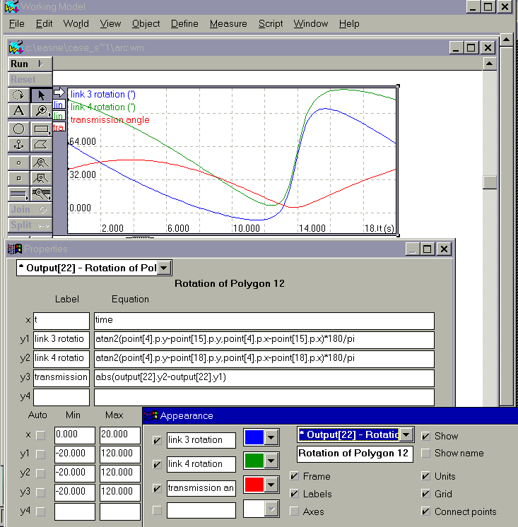
Figure 2: Properties and appearance menu for a customized output graph.
![]()
Copyright 1996, College of Engineering, University of Rhode Island